Portfolio optimization: Some aspects of modeling and computing

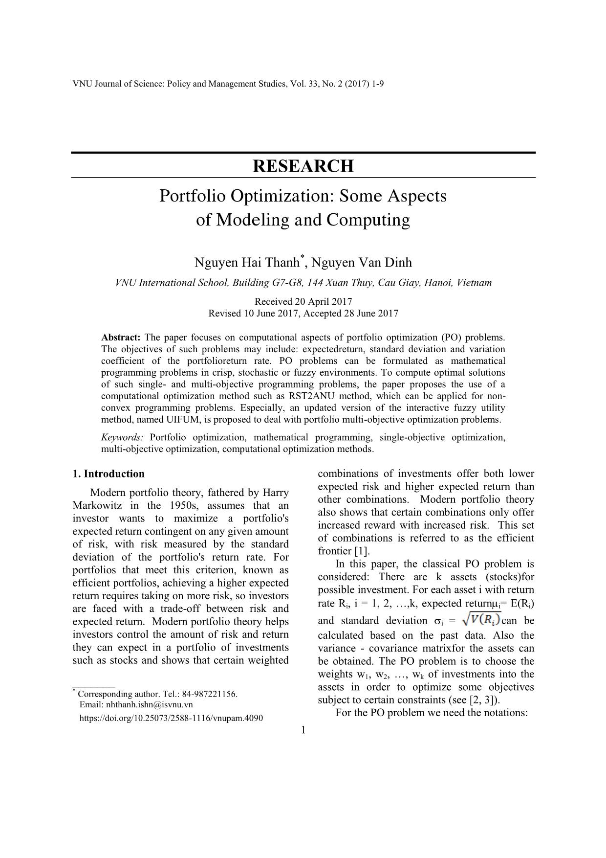
VNU Journal of Science: Policy and Management Studies, Vol. 33, No. 2 (2017) 1-9 
 1 
RESEARCH 
Portfolio Optimization: Some Aspects 
of Modeling and Computing 
Nguyen Hai Thanh*, Nguyen Van Dinh 
VNU International School, Building G7-G8, 144 Xuan Thuy, Cau Giay, Hanoi, Vietnam 
Received 20 April 2017 
Revised 10 June 2017, Accepted 28 June 2017 
Abstract: The paper focuses on computational aspects of portfolio optimization (PO) problems. 
The objectives of such problems may include: expectedreturn, standard deviation and variation 
coefficient of the portfolioreturn rate. PO problems can be formulated as mathematical 
programming problems in crisp, stochastic or fuzzy environments. To compute optimal solutions 
of such single- and multi-objective programming problems, the paper proposes the use of a 
computational optimization method such as RST2ANU method, which can be applied for non-
convex programming problems. Especially, an updated version of the interactive fuzzy utility 
method, named UIFUM, is proposed to deal with portfolio multi-objective optimization problems. 
Keywords: Portfolio optimization, mathematical programming, single-objective optimization, 
multi-objective optimization, computational optimization methods. 
1. Introduction
 *
Modern portfolio theory, fathered by Harry 
Markowitz in the 1950s, assumes that an 
investor wants to maximize a portfolio's 
expected return contingent on any given amount 
of risk, with risk measured by the standard 
deviation of the portfolio's return rate. For 
portfolios that meet this criterion, known as 
efficient portfolios, achieving a higher expected 
return requires taking on more risk, so investors 
are faced with a trade-off between risk and 
expected return. Modern portfolio theory helps 
investors control the amount of risk and return 
they can expect in a portfolio of investments 
such as stocks and shows that certain weighted 
_______ 
* Corresponding author. Tel.: 84-987221156. 
 Email: nhthanh.ishn@isvnu.vn 
 https://doi.org/10.25073/2588-1116/vnupam.4090 
combinations of investments offer both lower 
expected risk and higher expected return than 
other combinations. Modern portfolio theory 
also shows that certain combinations only offer 
increased reward with increased risk. This set 
of combinations is referred to as the efficient 
frontier [1]. 
In this paper, the classical PO problem is 
considered: There are k assets (stocks)for 
possible investment. For each asset i with return 
rate Ri, i = 1, 2, ,k, expected returni= E(Ri) 
and standard deviation i = can be 
calculated based on the past data. Also the 
variance - covariance matrixfor the assets can 
be obtained. The PO problem is to choose the 
weights w1, w2, , wk of investments into the 
assets in order to optimize some objectives 
subject to certain constraints (see [2, 3]). 
For the PO problem we need the notations: 
 N.H. Thanh, N.V. Dinh / VNU Journal of Science: Policy and Management Studies, Vol. 33, No. 2 (2017) 1-9 
2 
w = (w1, w2, , wk)
T
, 
 = (1, 2, ,k)
T
, 
and the variance - covariance matrix: 
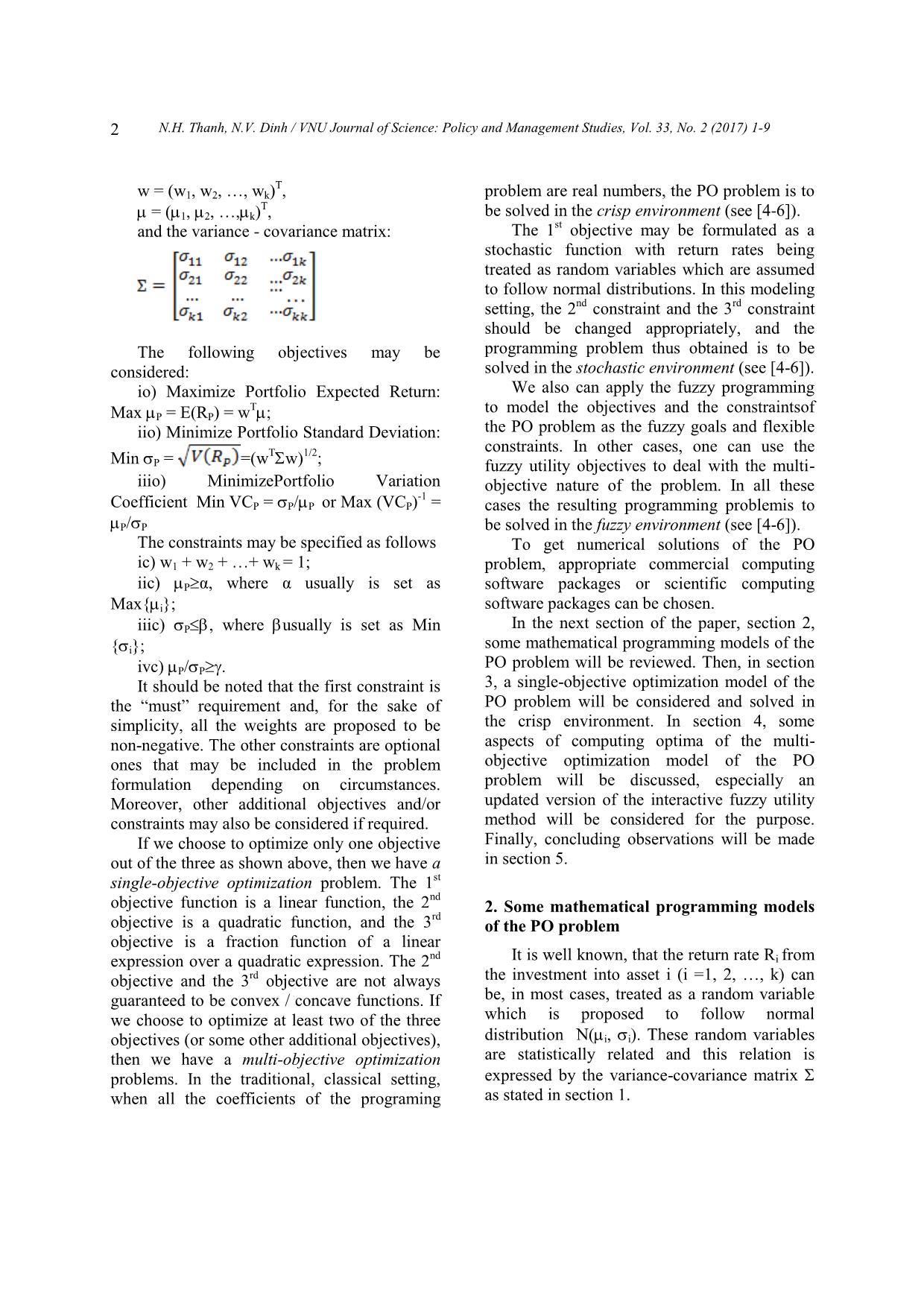
The following objectives may be 
considered: 
io) Maximize Portfolio Expected Return: 
Max P = E(RP) = w
T; 
iio) Minimize Portfolio Standard Deviation: 
Min P = =(w
Tw)1/2; 
iiio) MinimizePortfolio Variation 
Coefficient Min VCP = P/P or Max (VCP)
-1
 = 
P/P 
The constraints may be specified as follows 
ic) w1 + w2 + + wk = 1; 
iic) P α, where α usually is set as 
Max{i}; 
iiic) P , where usually is set as Min 
{i}; 
ivc) P/P . 
It should be noted that the first constraint is 
the “must” requirement and, for the sake of 
simplicity, all the weights are proposed to be 
non-negative. The other constraints are optional 
ones that may be included in the problem 
formulation depending on circumstances. 
Moreover, other additional objectives and/or 
constraints may also be considered if required. 
If we choose to optimize only one objective 
out of the three as shown above, then we have a 
single-objective optimization problem. The 1
st
objective function is a linear function, the 2
nd
objective is a quadratic function, and the 3
rd
objective is a fraction function of a linear 
expression over a quadratic expression. The 2
nd
objective and the 3
rd
 objective are not always 
guaranteed to be convex / concave functions. If 
we choose to optimize at least two of the three 
objectives (or some other additional objectives), 
then we have a multi-objective optimization 
problems. In the traditional, classical setting, 
when all the coefficients of the programing 
problem are real numbers, the PO problem is to 
be solved in the crisp environment (see [4-6]). 
The 1
st
 objective may be formulated as a 
stochastic function with return rates being 
treated as random variables which are assumed 
to follow normal distributions. In this modeling 
setti ...  2 (2017) 1-9 
4 
contain at least one non-linear function either in 
the objective or in the constraints, where there 
is the expression: 
Min P = (w
Tw)1/2 = 
=
Moreover, in most situations the variance-
covariance matrix is not a positive definite one, 
and the realistic problemsneed not to be of 
convex, concave or d.c. programming type (see 
[2, 3]). Therefore, most deterministic 
computational optimization methods can not 
guarantee to provide global optima but only 
local optima. Hence, in this paper we propose 
to use acomputational optimization method 
called RST2ANU method (see [5-7]) to compute 
the optima of PO problems 2a, 2b and 2c. 
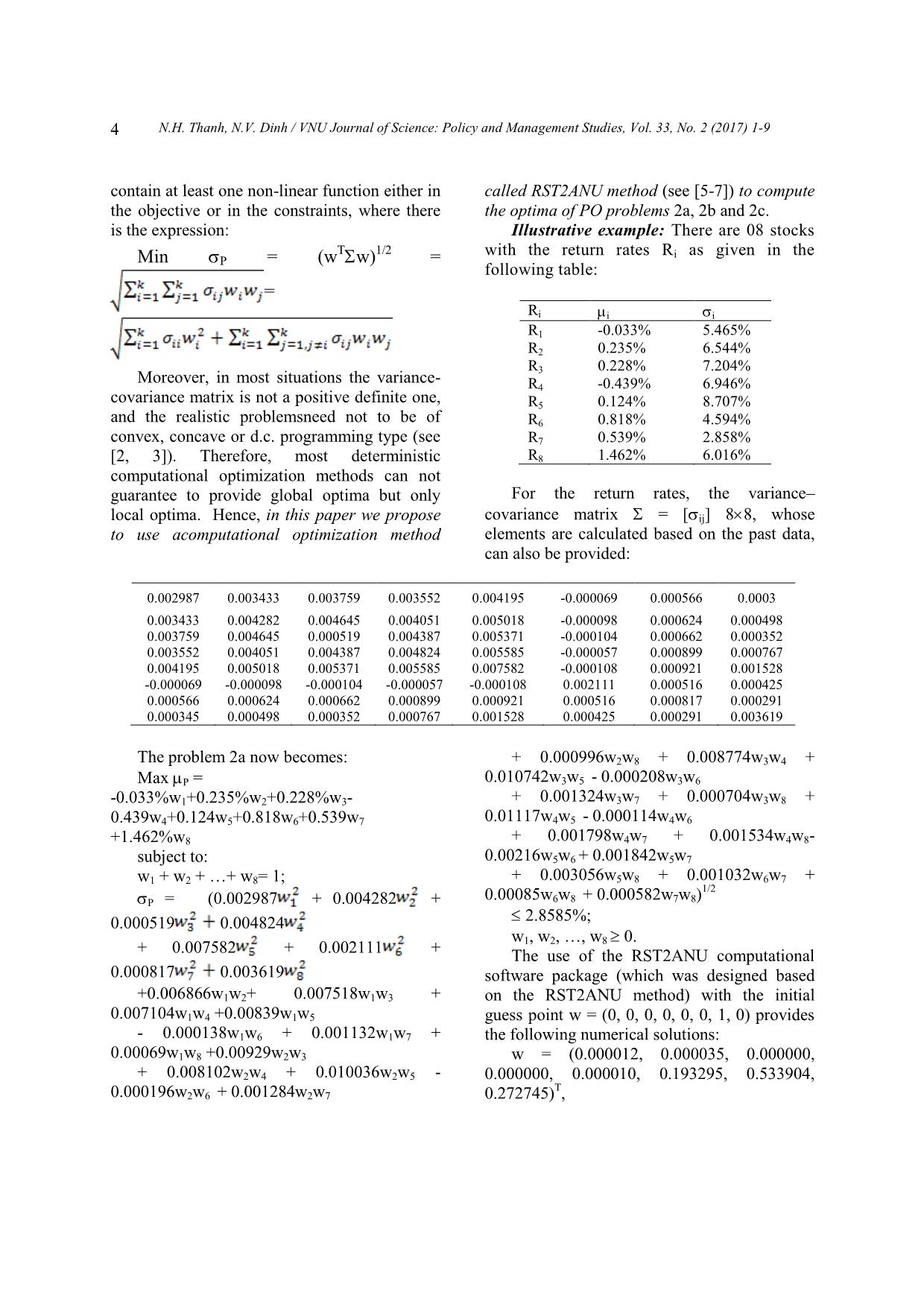
Illustrative example: There are 08 stocks 
with the return rates Ri as given in the 
following table: 
Ri i i 
R1 -0.033% 5.465% 
R2 0.235% 6.544% 
R3 0.228% 7.204% 
R4 -0.439% 6.946% 
R5 0.124% 8.707% 
R6 0.818% 4.594% 
R7 0.539% 2.858% 
R8 1.462% 6.016% 
For the return rates, the variance–
covariance matrix  = [ij] 8 8, whose 
elements are calculated based on the past data, 
can also be provided: 
f 
0.002987 0.003433 0.003759 0.003552 0.004195 -0.000069 0.000566 0.0003 
0.003433 0.004282 0.004645 0.004051 0.005018 -0.000098 0.000624 0.000498 
0.003759 0.004645 0.000519 0.004387 0.005371 -0.000104 0.000662 0.000352 
0.003552 0.004051 0.004387 0.004824 0.005585 -0.000057 0.000899 0.000767 
0.004195 0.005018 0.005371 0.005585 0.007582 -0.000108 0.000921 0.001528 
-0.000069 -0.000098 -0.000104 -0.000057 -0.000108 0.002111 0.000516 0.000425 
0.000566 0.000624 0.000662 0.000899 0.000921 0.000516 0.000817 0.000291 
0.000345 0.000498 0.000352 0.000767 0.001528 0.000425 0.000291 0.003619 
g 
The problem 2a now becomes: 
Max P = 
-0.033%w1+0.235%w2+0.228%w3-
0.439w4+0.124w5+0.818w6+0.539w7 
+1.462%w8 
subject to: 
w1 + w2 + + w8= 1; 
P = (0.002987 + 0.004282 + 
0.000519 0.004824 
+ 0.007582 + 0.002111 + 
0.000817 0.003619 
+0.006866w1w2+ 0.007518w1w3 + 
0.007104w1w4 +0.00839w1w5 
- 0.000138w1w6 + 0.001132w1w7 + 
0.00069w1w8 +0.00929w2w3 
+ 0.008102w2w4 + 0.010036w2w5 - 
0.000196w2w6 + 0.001284w2w7 
+ 0.000996w2w8 + 0.008774w3w4 + 
0.010742w3w5 - 0.000208w3w6 
+ 0.001324w3w7 + 0.000704w3w8 + 
0.01117w4w5 - 0.000114w4w6
+ 0.001798w4w7 + 0.001534w4w8- 
0.00216w5w6 + 0.001842w5w7 
+ 0.003056w5w8 + 0.001032w6w7 + 
0.00085w6w8 + 0.000582w7w8)
1/2
 2.8585%; 
w1, w2, , w8 0. 
The use of the RST2ANU computational 
software package (which was designed based 
on the RST2ANU method) with the initial 
guess point w = (0, 0, 0, 0, 0, 0, 1, 0) provides 
the following numerical solutions: 
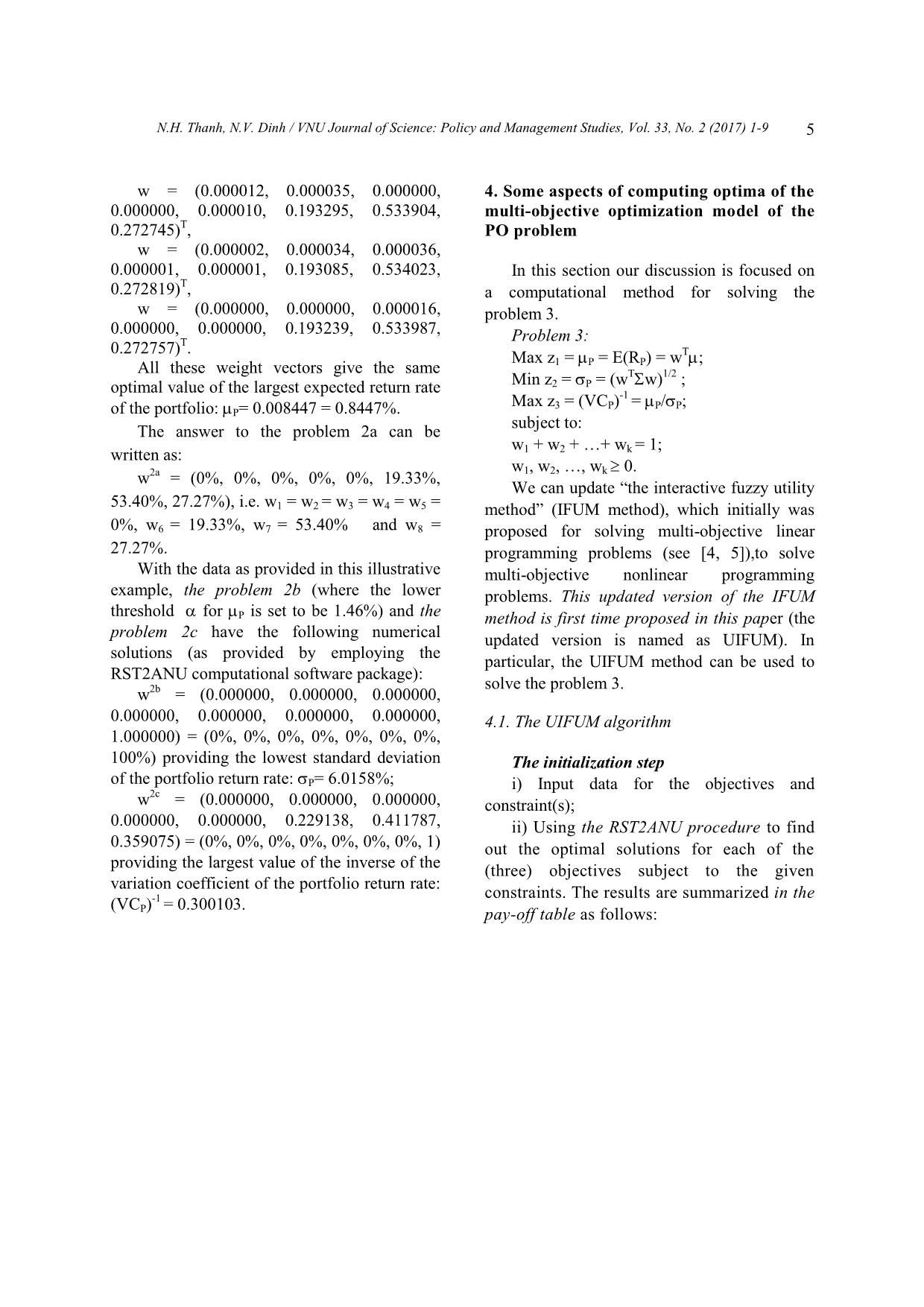
w = (0.000012, 0.000035, 0.000000, 
0.000000, 0.000010, 0.193295, 0.533904, 
0.272745)
T
, 
N.H. Thanh, N.V. Dinh / VNU Journal of Science: Policy and Management Studies, Vol. 33, No. 2 (2017) 1-9 5 
w = (0.000012, 0.000035, 0.000000, 
0.000000, 0.000010, 0.193295, 0.533904, 
0.272745)
T
, 
w = (0.000002, 0.000034, 0.000036, 
0.000001, 0.000001, 0.193085, 0.534023, 
0.272819)
T
, 
w = (0.000000, 0.000000, 0.000016, 
0.000000, 0.000000, 0.193239, 0.533987, 
0.272757)
T
. 
All these weight vectors give the same 
optimal value of the largest expected return rate 
of the portfolio: P= 0.008447 = 0.8447%. 
The answer to the problem 2a can be 
written as: 
w
2a
 = (0%, 0%, 0%, 0%, 0%, 19.33%, 
53.40%, 27.27%), i.e. w1 = w2 = w3 = w4 = w5 = 
0%, w6 = 19.33%, w7 = 53.40% and w8 = 
27.27%. 
With the data as provided in this illustrative 
example, the problem 2b (where the lower 
threshold for P is set to be 1.46%) and the 
problem 2c have the following numerical 
solutions (as provided by employing the 
RST2ANU computational software package): 
w
2b
 = (0.000000, 0.000000, 0.000000, 
0.000000, 0.000000, 0.000000, 0.000000, 
1.000000) = (0%, 0%, 0%, 0%, 0%, 0%, 0%, 
100%) providing the lowest standard deviation 
of the portfolio return rate: P= 6.0158%; 
w
2c
 = (0.000000, 0.000000, 0.000000, 
0.000000, 0.000000, 0.229138, 0.411787, 
0.359075) = (0%, 0%, 0%, 0%, 0%, 0%, 0%, 1) 
providing the largest value of the inverse of the 
variation coefficient of the portfolio return rate: 
(VCP)
-1 
= 0.300103. 
4. Some aspects of computing optima of the 
multi-objective optimization model of the 
PO problem 
In this section our discussion is focused on 
a computational method for solving the 
problem 3. 
Problem 3: 
Max z1 = P = E(RP) = w
T; 
Min z2 = P = (w
Tw)1/2 ; 
Max z3 = (VCP)
-1 
= P/P; 
subject to: 
w1 + w2 + + wk = 1; 
w1, w2, , wk 0. 
We can update “the interactive fuzzy utility 
method” (IFUM method), which initially was 
proposed for solving multi-objective linear 
programming problems (see [4, 5]),to solve 
multi-objective nonlinear programming 
problems. This updated version of the IFUM 
method is first time proposed in this paper (the 
updated version is named as UIFUM). In 
particular, the UIFUM method can be used to 
solve the problem 3. 
4.1. The UIFUM algorithm 
The initialization step 
i) Input data for the objectives and 
constraint(s); 
ii) Using the RST2ANU procedure to find 
out the optimal solutions for each of the 
(three) objectives subject to the given 
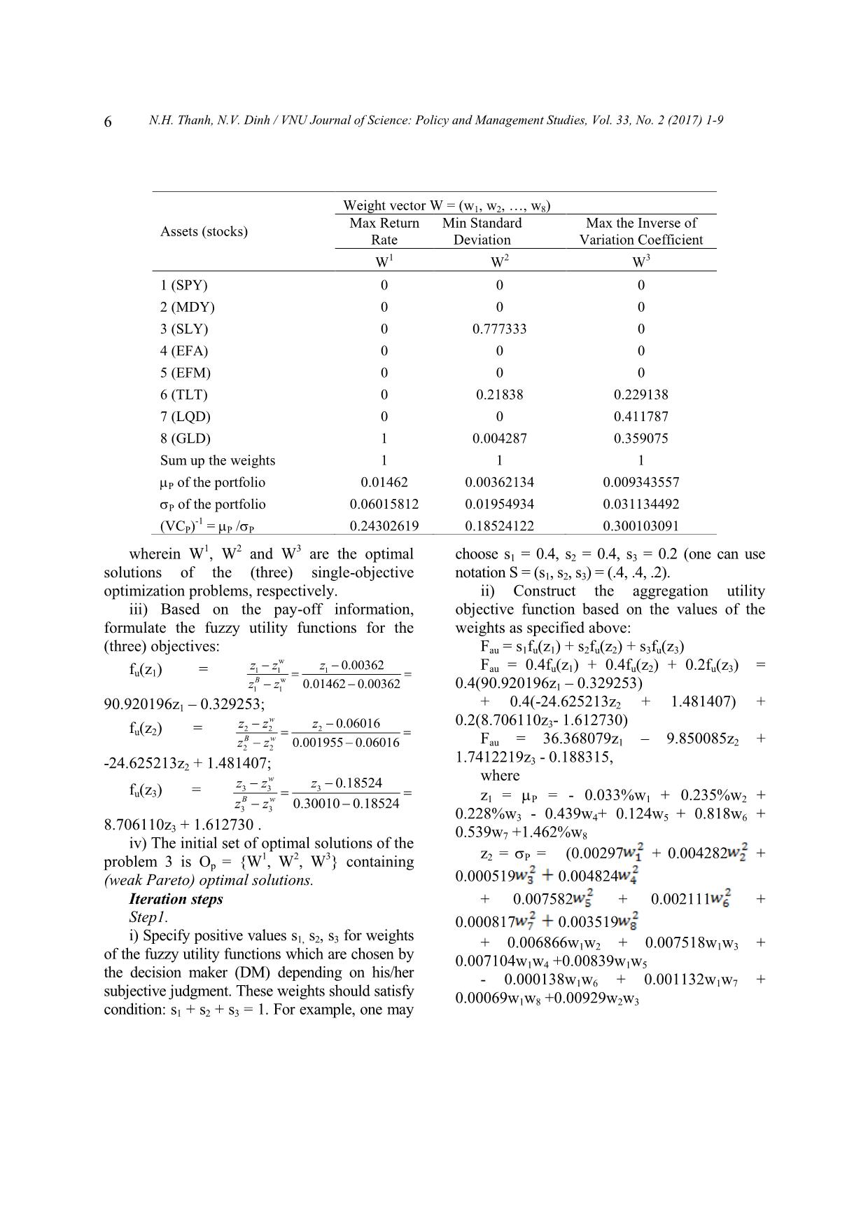
constraints. The results are summarized in the 
pay-off table as follows: 
f 
 N.H. Thanh, N.V. Dinh / VNU Journal of Science: Policy and Management Studies, Vol. 33, No. 2 (2017) 1-9 
6 
wherein W
1
, W
2
 and W
3
 are the optimal 
solutions of the (three) single-objective 
optimization problems, respectively. 
iii) Based on the pay-off information, 
formulate the fuzzy utility functions for the 
(three) objectives: 
fu(z1) = 
w
1 1 1
w
1 1
0.00362
0.01462 0.00362B
z z z
z z
90.920196z1 – 0.329253; 
fu(z2) = 2 2 2
2 2
0.06016
0.001955 0.06016
w
B w
z z z
z z
-24.625213z2 + 1.481407; 
fu(z3) = 3 3 3
3 3
0.18524
0.30010 0.18524
w
B w
z z z
z z
8.706110z3 + 1.612730 . 
iv) The initial set of optimal solutions of the 
problem 3 is Op = {W
1
, W
2
, W
3
} containing 
(weak Pareto) optimal solutions. 
Iteration steps 
Step1. 
i) Specify positive values s1, s2, s3 for weights 
of the fuzzy utility functions which are chosen by 
the decision maker (DM) depending on his/her 
subjective judgment. These weights should satisfy 
condition: s1 + s2 + s3 = 1. For example, one may 
choose s1 = 0.4, s2 = 0.4, s3 = 0.2 (one can use 
notation S = (s1, s2, s3) = (.4, .4, .2). 
ii) Construct the aggregation utility 
objective function based on the values of the 
weights as specified above: 
Fau = s1fu(z1) + s2fu(z2) + s3fu(z3) 
Fau = 0.4fu(z1) + 0.4fu(z2) + 0.2fu(z3) = 
0.4(90.920196z1 – 0.329253) 
+ 0.4(-24.625213z2 + 1.481407) + 
0.2(8.706110z3- 1.612730) 
Fau = 36.368079z1 – 9.850085z2 + 
1.7412219z3 - 0.188315, 
where 
z1 = P = - 0.033%w1 + 0.235%w2 + 
0.228%w3 - 0.439w4+ 0.124w5 + 0.818w6 + 
0.539w7 +1.462%w8 
z2 = P = (0.00297 + 0.004282 + 
0.000519 0.004824 
+ 0.007582 + 0.002111 + 
0.000817 0.003519 
+ 0.006866w1w2 + 0.007518w1w3 + 
0.007104w1w4 +0.00839w1w5 
- 0.000138w1w6 + 0.001132w1w7 + 
0.00069w1w8 +0.00929w2w3 
Assets (stocks) 
Weight vector W = (w1, w2, , w8) 
Max Return 
Rate 
Min Standard 
Deviation 
Max the Inverse of 
Variation Coefficient 
W
1
 W
2
 W
3
1 (SPY) 0 0 0 
2 (MDY) 0 0 0 
3 (SLY) 0 0.777333 0 
4 (EFA) 0 0 0 
5 (EFM) 0 0 0 
6 (TLT) 0 0.21838 0.229138 
7 (LQD) 0 0 0.411787 
8 (GLD) 1 0.004287 0.359075 
Sum up the weights 1 1 1 
P of the portfolio 0.01462 0.00362134 0.009343557 
P of the portfolio 0.06015812 0.01954934 0.031134492 
(VCP)
-1
 = P /P 0.24302619 0.18524122 0.300103091 
N.H. Thanh, N.V. Dinh / VNU Journal of Science: Policy and Management Studies, Vol. 33, No. 2 (2017) 1-9 7 
+ 0.008102w2w4 + 0.010036w2w5 - 
0.000196w2w6 + 0.001284w2w7 
+ 0.000996w2w8 + 0.008774w3w4 + 
0.010742w3w5 - 0.000208w3w6
+ 0.001324w3w7 + 0.000704w3w8 + 
0.01117w4w5 - 0.000114w4w6 
+ 0.001798w4w7 + 0.001534w4w8 - 
0.00216w5w6 + 0.001842w5w7 
+ 0.003056w5w8 + 0.001032w6w7 + 
0.00085w6w8 + 0.000582w7w8)
1/2
z3 = P / P . 
Step2. 
i) Using the RST2ANU procedure to find 
out the optimal solution of the obtained single-
objective programming problem: 
Max Fau = 36.368079z1 – 9.850085z2 + 
1.7412219z3 - 0.188315; 
subject to: 
w1 + w2 + + wk = 1; 
w1, w2, , wk 0. 
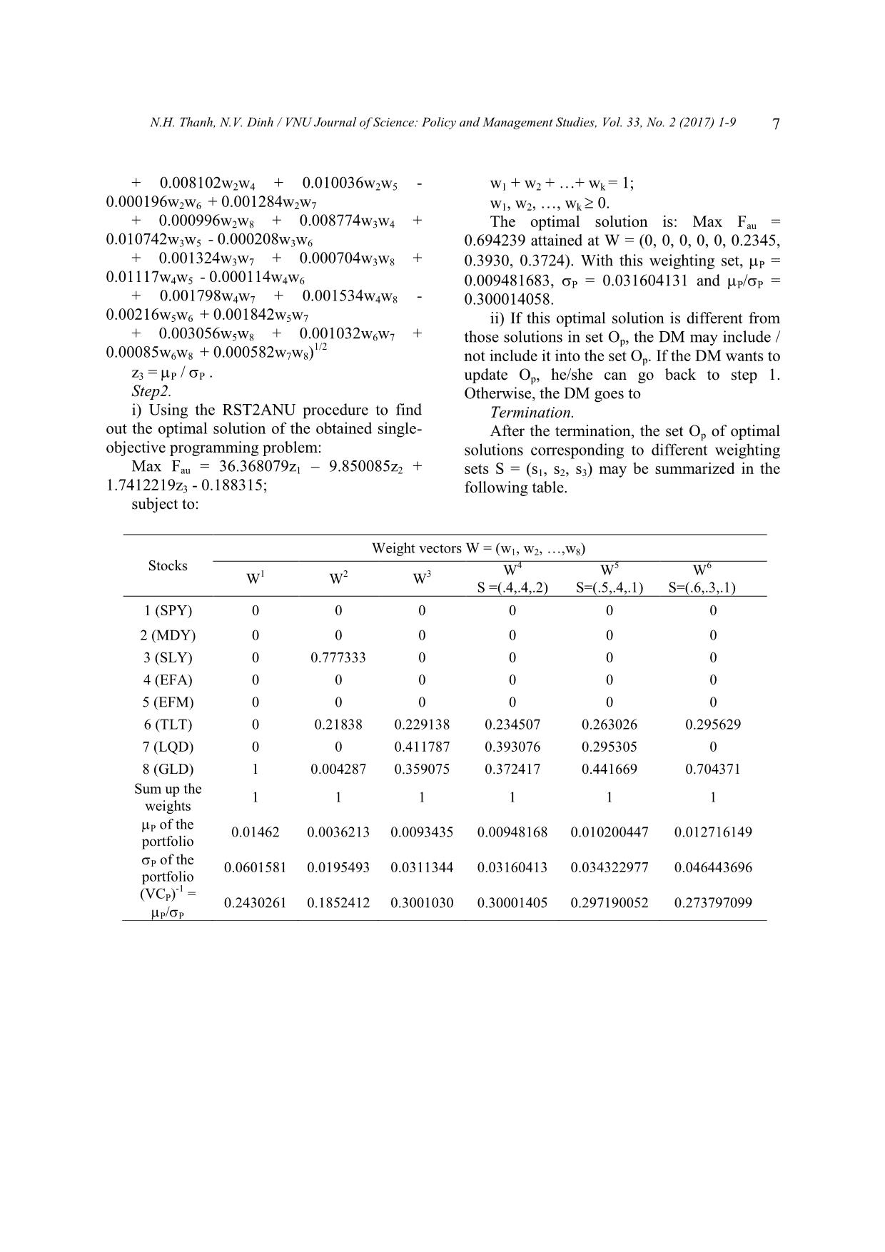
The optimal solution is: Max Fau = 
0.694239 attained at W = (0, 0, 0, 0, 0, 0.2345, 
0.3930, 0.3724). With this weighting set, P = 
0.009481683, P = 0.031604131 and P/P = 
0.300014058. 
ii) If this optimal solution is different from 
those solutions in set Op, the DM may include / 
not include it into the set Op. If the DM wants to 
update Op, he/she can go back to step 1. 
Otherwise, the DM goes to 
Termination. 
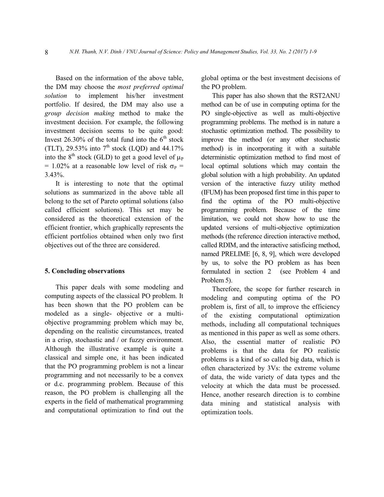
After the termination, the set Op of optimal 
solutions corresponding to different weighting 
sets S = (s1, s2, s3) may be summarized in the 
following table. 
D 
r 
Stocks 
Weight vectors W = (w1, w2, ,w8) 
W
1
 W
2
 W
3
W
4
S =(.4,.4,.2) 
W
5
S=(.5,.4,.1) 
W
6
S=(.6,.3,.1) 
1 (SPY) 0 0 0 0 0 0 
2 (MDY) 0 0 0 0 0 0 
3 (SLY) 0 0.777333 0 0 0 0 
4 (EFA) 0 0 0 0 0 0 
5 (EFM) 0 0 0 0 0 0 
6 (TLT) 0 0.21838 0.229138 0.234507 0.263026 0.295629 
7 (LQD) 0 0 0.411787 0.393076 0.295305 0 
8 (GLD) 1 0.004287 0.359075 0.372417 0.441669 0.704371 
Sum up the 
weights 
1 1 1 1 1 1 
P of the 
portfolio 
0.01462 0.0036213 0.0093435 0.00948168 0.010200447 0.012716149 
P of the 
portfolio 
0.0601581 0.0195493 0.0311344 0.03160413 0.034322977 0.046443696 
(VCP)
-1
 = 
P/P 
0.2430261 0.1852412 0.3001030 0.30001405 0.297190052 0.273797099 
 N.H. Thanh, N.V. Dinh / VNU Journal of Science: Policy and Management Studies, Vol. 33, No. 2 (2017) 1-9 
8 
Based on the information of the above table, 
the DM may choose the most preferred optimal 
solution to implement his/her investment 
portfolio. If desired, the DM may also use a 
group decision making method to make the 
investment decision. For example, the following 
investment decision seems to be quite good: 
Invest 26.30% of the total fund into the 6
th
 stock 
(TLT), 29.53% into 7
th
 stock (LQD) and 44.17% 
into the 8
th
 stock (GLD) to get a good level of P 
= 1.02% at a reasonable low level of risk P = 
3.43%. 
It is interesting to note that the optimal 
solutions as summarized in the above table all 
belong to the set of Pareto optimal solutions (also 
called efficient solutions). This set may be 
considered as the theoretical extension of the 
efficient frontier, which graphically represents the 
efficient portfolios obtained when only two first 
objectives out of the three are considered. 
5. Concluding observations 
This paper deals with some modeling and 
computing aspects of the classical PO problem. It 
has been shown that the PO problem can be 
modeled as a single- objective or a multi-
objective programming problem which may be, 
depending on the realistic circumstances, treated 
in a crisp, stochastic and / or fuzzy environment. 
Although the illustrative example is quite a 
classical and simple one, it has been indicated 
that the PO programming problem is not a linear 
programming and not necessarily to be a convex 
or d.c. programming problem. Because of this 
reason, the PO problem is challenging all the 
experts in the field of mathematical programming 
and computational optimization to find out the 
global optima or the best investment decisions of 
the PO problem. 
This paper has also shown that the RST2ANU 
method can be of use in computing optima for the 
PO single-objective as well as multi-objective 
programming problems. The method is in nature a 
stochastic optimization method. The possibility to 
improve the method (or any other stochastic 
method) is in incorporating it with a suitable 
deterministic optimization method to find most of 
local optimal solutions which may contain the 
global solution with a high probability. An updated 
version of the interactive fuzzy utility method 
(IFUM) has been proposed first time in this paper to 
find the optima of the PO multi-objective 
programming problem. Because of the time 
limitation, we could not show how to use the 
updated versions of multi-objective optimization 
methods (the reference direction interactive method, 
called RDIM, and the interactive satisficing method, 
named PRELIME [6, 8, 9], which were developed 
by us, to solve the PO problem as has been 
formulated in section 2 (see Problem 4 and 
Problem 5). 
Therefore, the scope for further research in 
modeling and computing optima of the PO 
problem is, first of all, to improve the efficiency 
of the existing computational optimization 
methods, including all computational techniques 
as mentioned in this paper as well as some others. 
Also, the essential matter of realistic PO 
problems is that the data for PO realistic 
problems is a kind of so called big data, which is 
often characterized by 3Vs: the extreme volume 
of data, the wide variety of data types and the 
velocity at which the data must be processed. 
Hence, another research direction is to combine 
data mining and statistical analysis with 
optimization tools. 
N.H. Thanh, N.V. Dinh / VNU Journal of Science: Policy and Management Studies, Vol. 33, No. 2 (2017) 1-9 9 
References 
[1] Sabbadini, Tony, Manufacturing Portfolio 
Theory, International Institute for Advanced 
Studies in Systems Research and Cybernetics, 
working paper, 2010. 
[2] Wai-Sum Chan and Yiu-KuenTse, Financial 
Mathematics for Actuaries, Updated Edition, 
McGraw - Hill Education, Singapore, 2013. 
[3] Jaehyun Park, Ahmed Bou-Rabee and Stephen 
Boyd, Portfolio Optimization, EE103 Stanford 
University Lecture note, 2014. 
[4] Nguyen Hai Thanh, Applied Mathematics (in 
Vietnamese), The Hanoi National University of 
Education’s Publishing House, Hanoi, 2005. 
[5] Nguyen Hai Thanh, Optimization (in Vietnamese), 
The Hanoi University of Science and Technology’s 
Publishing House, Hanoi, 2006. 
[6] Nguyen Hai Thanh, Optimization in Fuzzy-
Stochastic Environment and its Applications in 
Industry and Economics, Internationalization 
Studies, 1 (2012), 131. 
[7] Chander Mohan, Nguyen Hai Thanh, A 
Controlled Random Search Technique 
Incorporating the Simulated Annealing Concept 
for Solving Integer and Mixed Integer Global 
Optimization Problems, Computational 
Optimization and Applications, 14 (1999), 103. 
[8] Chander Mohan, Nguyen Hai Thanh, Reference 
Direction Method for Solving Multi-objective 
Fuzzy Programming, European Journal of 
Operational Research, 107 (1998), 599. 
[9] Chander Mohan, Nguyen Hai Thanh, An 
Interactive Satisficing Method for Solving Multi-
objective Mixed Fuzzy-Stochastic Programming 
Problems, International Journal for Fuzzy Sets and 
Systems, 117 (2001), 61. 
T 
g