Performance analysis of global - local mean square error criterion of stochastic linearization for nonlinear oscillators
One popular class of methods for approximate solutions of nonlinear systems under
random excitations is GEL techniques, which are most used in structural dynamics and in
the engineering mechanics applications. This is partially due to its simplicity and applicability to systems with MDOF, and ones under various types of random excitations. The
key idea of GEL is to replace the nonlinear system by a linear one such that the behavior of the equivalent linear system approximates that of the original nonlinear oscillator.
The standard way is that the coefficients of linearization are to be found by the classical
mean square error criterion [1,2]. Although the method is very efficient, but its accuracy
decreases as the nonlinearity increases and in many cases it gives very larger errors due
to the non-Gaussian property of the response. That is reason why many researches have
been done in recent decades on improving GEL, for example [3–11]. One among them
is LOMSEC that was first proposed by N. D. Anh and Di Paola [10], and then further
developed by N. D. Anh and L. X. Hung [11]. The basic difference of LOMSEC from the
classical GEL is that the integration domain for mean square of response taken over finite
one (local one) instead of (−¥, ¥) in the classical GEL. As LOMSEC can give a good improvement on accuracy, however, the local integration domain in question was unknown
and it has resulted in the main disadvantage of LOMSEC. Recently a dual conception was
proposed in the study of responses to nonlinear systems [12, 13]. One remarkable advantage of the dual conception is its consideration of two different aspects of a problem in
question allows the investigation to be more appropriate. Applying the dual approach
to LOMSEC, a new criterion namely global-local mean square error criterion (GLOMSEC) has been recently proposed L. X. Hung et al. [14, 15]for nonlinear systems under
white noise excitation, in which new values of linearization coefficients are obtained as
global averaged values of all local linearization coefficients. This paper is an additional
research to aim at evaluating the improved performance of the proposed criterion; herein
we analyse two more applications, which are a rolling ship oscillation and two-degreeof-freedom one. The results show a significant improvement on accuracy of solutions by
the new criterion compared to the ones by the classical GEL.
Trang 1
Trang 2
Trang 3
Trang 4
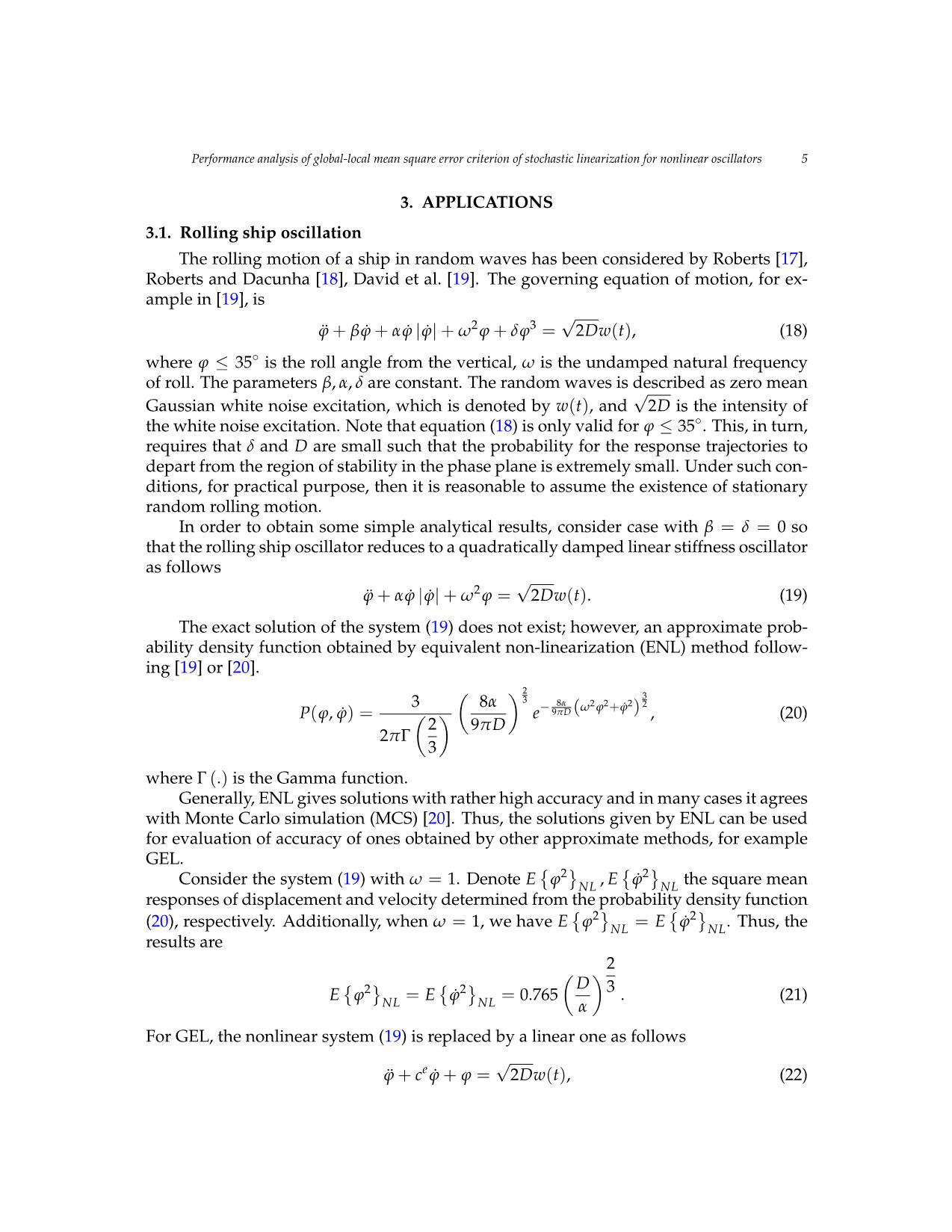
Trang 5
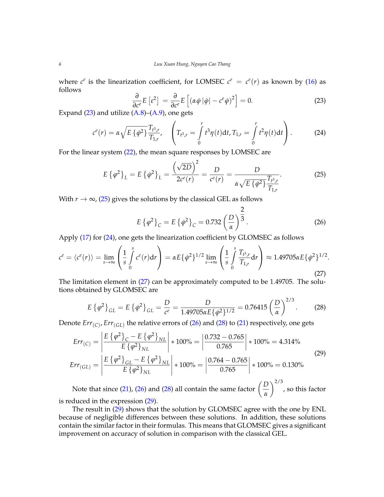
Trang 6
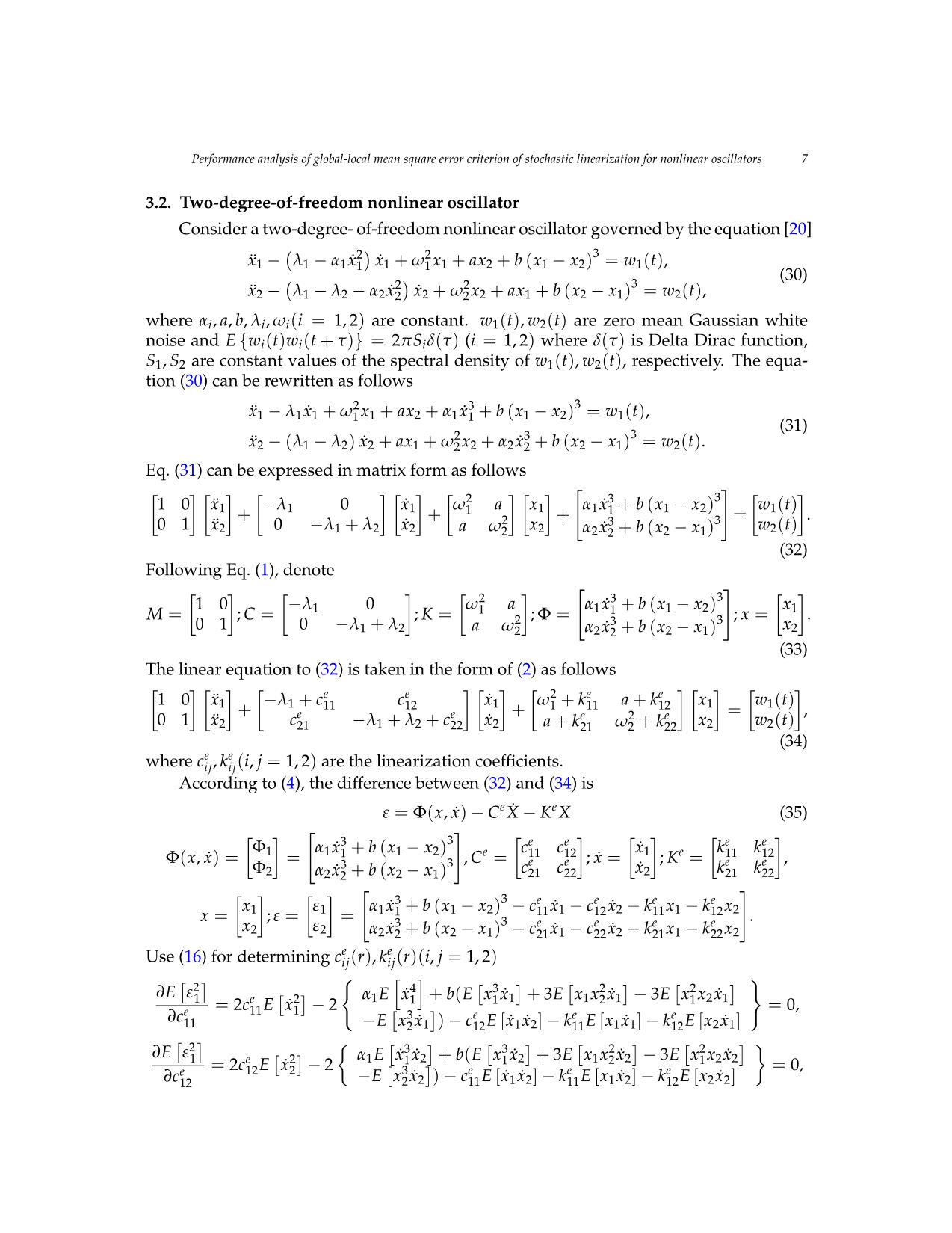
Trang 7
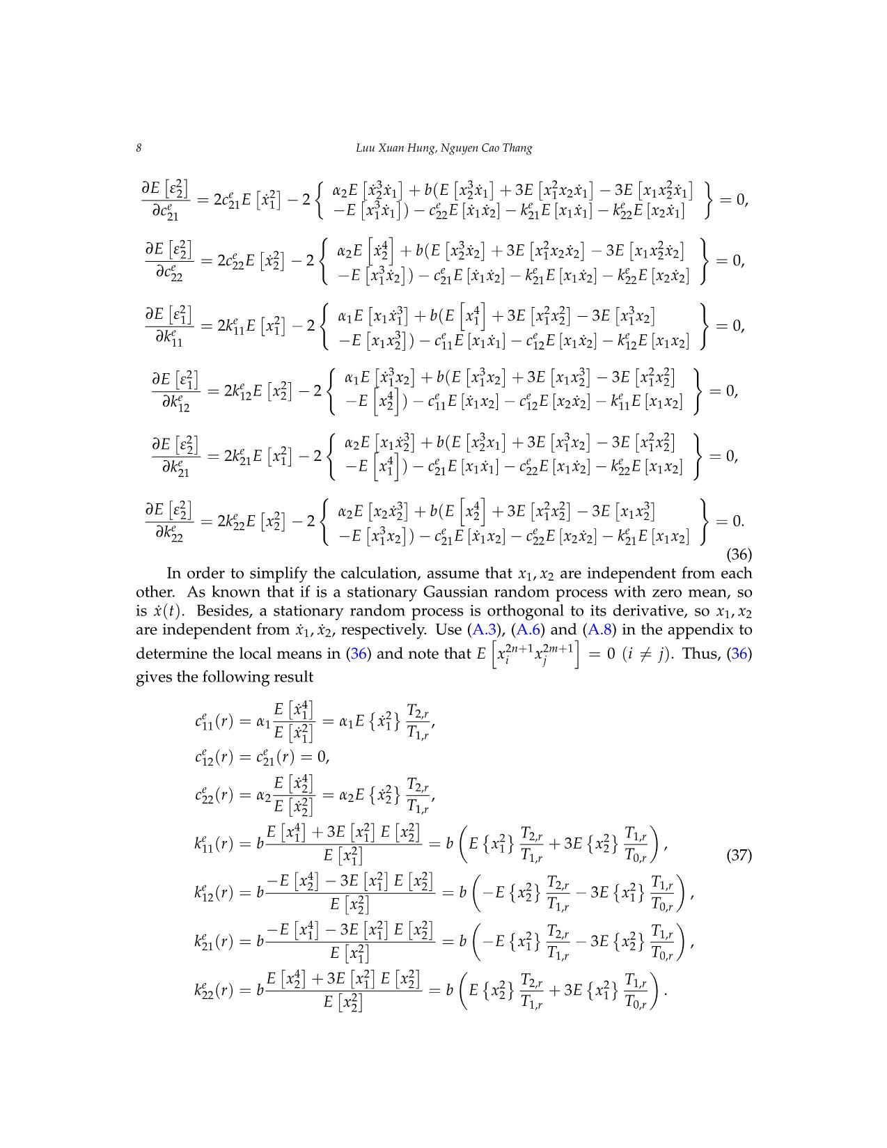
Trang 8
Trang 9
Trang 10
Tải về để xem bản đầy đủ
Tóm tắt nội dung tài liệu: Performance analysis of global - local mean square error criterion of stochastic linearization for nonlinear oscillators
Vietnam Journal of Mechanics, VAST, Vol.41, No. 1 (2019), pp. 1 – 15
DOI: https://doi.org/10.15625/0866-7136/12015
PERFORMANCE ANALYSIS OF GLOBAL-LOCAL
MEAN SQUARE ERROR CRITERION OF STOCHASTIC
LINEARIZATION FOR NONLINEAR OSCILLATORS
Luu Xuan Hung1,2, Nguyen Cao Thang2,3,∗
1Hanoi Metropolitan Rail Board, Vietnam
2Institute of Mechanics, VAST, Hanoi, Vietnam
3Graduate University of Science and Technology, VAST, Hanoi, Vietnam
∗E-mail: caothang2002us@yahoo.com
Received: 22 March 2018 / Published online: 14 February 2019
Abstract. The paper presents a performance analysis of global-local mean square error
criterion of stochastic linearization for some nonlinear oscillators. This criterion of sto-
chastic linearization for nonlinear oscillators bases on dual conception to the local mean
square error criterion (LOMSEC). The algorithm is generally built to multi-degree of free-
dom (MDOF) nonlinear oscillators. Then, the performance analysis is carried out for two
applications which comprise a rolling ship oscillation and two-degree of freedom one. The
improvement on accuracy of the proposed criterion has been shown in comparison with
the conventional Gaussian equivalent linearization (GEL).
Keywords: probability; random; frequency response function; iteration method; mean
square.
1. INTRODUCTION
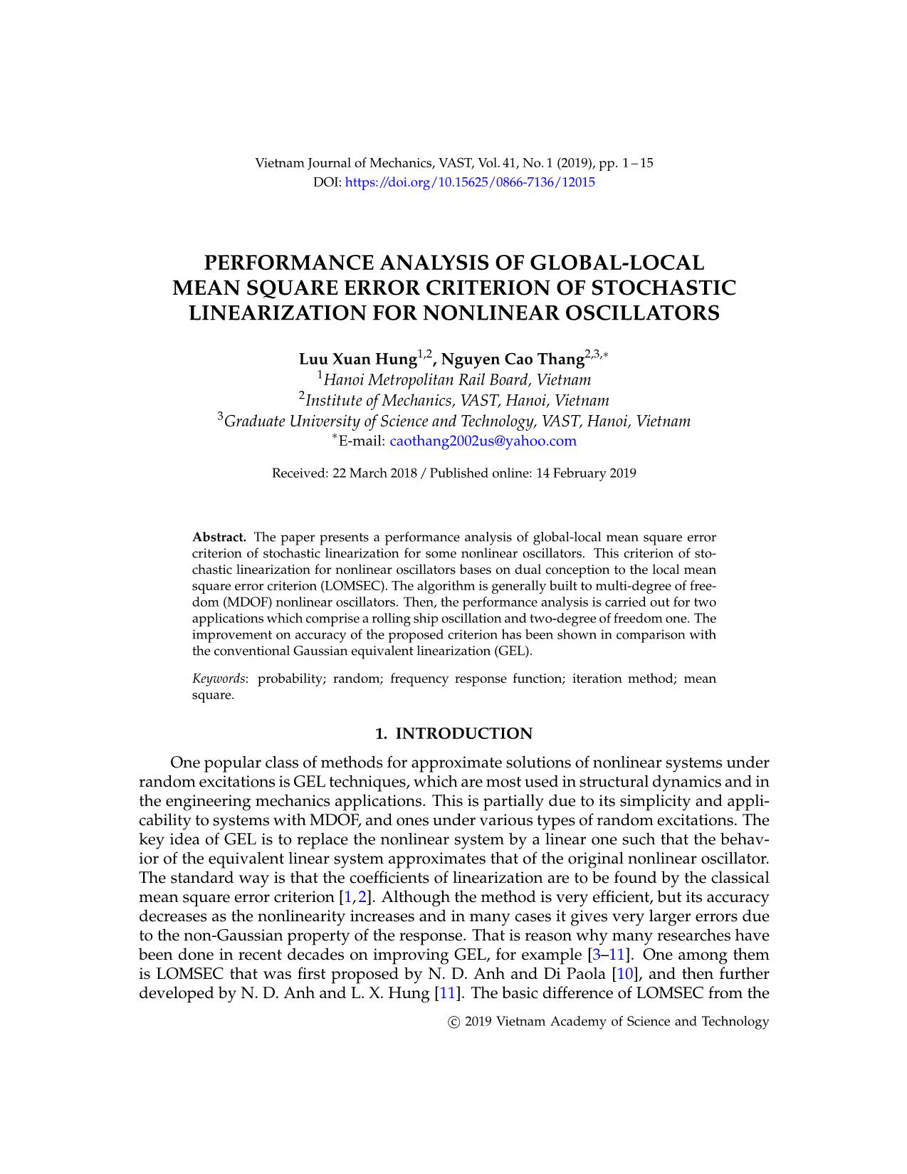
One popular class of methods for approximate solutions of nonlinear systems under
random excitations is GEL techniques, which are most used in structural dynamics and in
the engineering mechanics applications. This is partially due to its simplicity and appli-
cability to systems with MDOF, and ones under various types of random excitations. The
key idea of GEL is to replace the nonlinear system by a linear one such that the behav-
ior of the equivalent linear system approximates that of the original nonlinear oscillator.
The standard way is that the coefficients of linearization are to be found by the classical
mean square error criterion [1,2]. Although the method is very efficient, but its accuracy
decreases as the nonlinearity increases and in many cases it gives very larger errors due
to the non-Gaussian property of the response. That is reason why many researches have
been done in recent decades on improving GEL, for example [3–11]. One among them
is LOMSEC that was first proposed by N. D. Anh and Di Paola [10], and then further
developed by N. D. Anh and L. X. Hung [11]. The basic difference of LOMSEC from the
c 2019 Vietnam Academy of Science and Technology
2 Luu Xuan Hung, Nguyen Cao Thang
classical GEL is that the integration domain for mean square of response taken over finite
one (local one) instead of (−∞, ∞) in the classical GEL. As LOMSEC can give a good im-
provement on accuracy, however, the local integration domain in question was unknown
and it has resulted in the main disadvantage of LOMSEC. Recently a dual conception was
proposed in the study of responses to nonlinear systems [12,13]. One remarkable advan-
tage of the dual conception is its consideration of two different aspects of a problem in
question allows the investigation to be more appropriate. Applying the dual approach
to LOMSEC, a new criterion namely global-local mean square error criterion (GLOM-
SEC) has been recently proposed L. X. Hung et al. [14, 15]for nonlinear systems under
white noise excitation, in which new values of linearization coefficients are obtained as
global averaged values of all local linearization coefficients. This paper is an additional
research to aim at evaluating the improved performance of the proposed criterion; herein
we analyse two more applications, which are a rolling ship oscillation and two-degree-
of-freedom one. The results show a significant improvement on accuracy of solutions by
the new criterion compared to the ones by the classical GEL.
2. FORMULATION
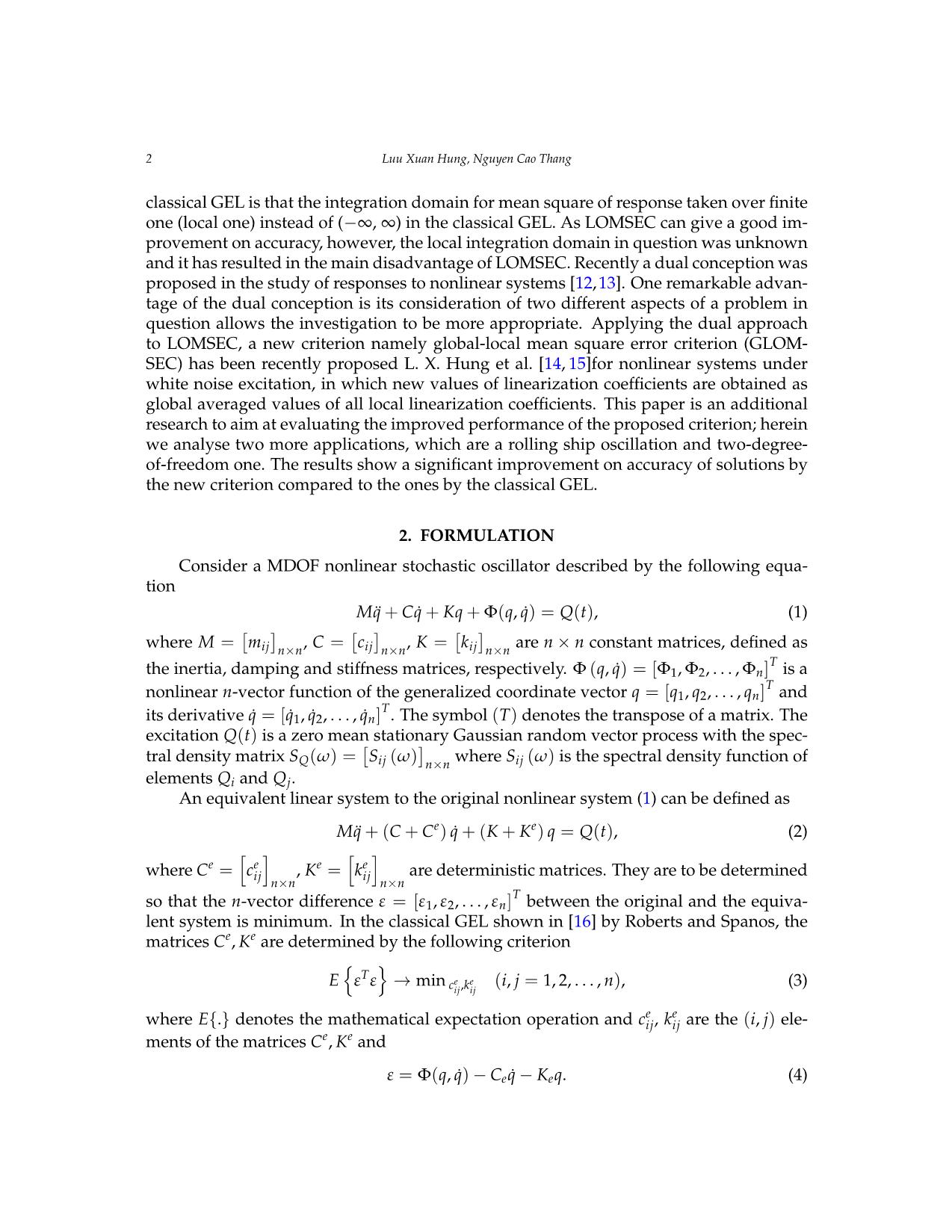
Consider a MDOF nonlinear stochastic oscillator described by the following equa-
tion
Mq¨ + Cq˙ + Kq + Φ(q, q˙) = Q(t), (1)
= = = ×
where M mij n×n, C cij n×n, K kij n×n are n n constant matrices, defined as
T
the inertia, damping and stiffness matrices, respectively. Φ (q, q˙) = [Φ1, Φ2,..., Φn] is a
T
nonlinear n-vector function of the generalized coordinate vector q = [q1, q2,..., qn] and
T
its derivative q˙ = [q˙1, q˙2,..., q˙n] . The symbol (T) denotes the transpose of a matrix. The
excitation Q(t) is a zero mean stationary Gaussian random vector process with the spec-
( ) = ( ) ( )
tral density matrix SQ ω Sij ω n×n where Sij ω is the spectral density function of
elements Qi and Qj.
An equivalent linear system to the original nonlinear system (1) can be defined as
Mq¨ + (C + Ce) q˙ + (K + Ke) q = Q(t), (2)
e h e i e h e i
where C = cij , K = kij are deterministic matrices. They are to be determined
n×n n×n
T
so that the n-vector difference ε = [ε1, ε2,..., εn] between the original and the equiva-
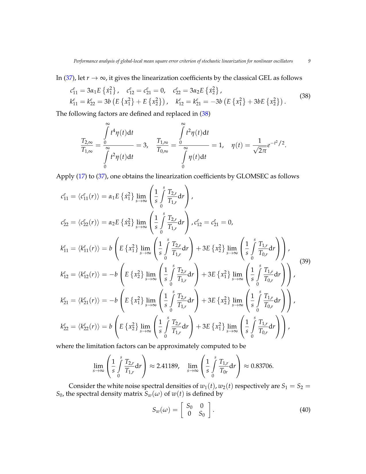
lent system is minimum. In the c ... α2E x˙2 lim dr , c12 = c21 = 0,
s→∞ s T1,r
0
s s
Z Z
e e 2 1 T2,r 2 1 T1,r
k11 = hk11(r)i = b E x1 lim dr + 3E x2 lim dr ,
s→∞ s T1,r s→∞ s T0,r
0 0
(39)
s s
Z Z
e e 2 1 T2,r 2 1 T1,r
k12 = hk12(r)i = −b E x2 lim dr + 3E x1 lim dr ,
s→∞ s T1,r s→∞ s T0,r
0 0
s s
Z Z
e e 2 1 T2,r 2 1 T1,r
k21 = hk21(r)i = −b E x1 lim dr + 3E x2 lim dr ,
s→∞ s T1,r s→∞ s T0,r
0 0
s s
Z Z
e e 2 1 T2,r 2 1 T1,r
k22 = hk22(r)i = b E x2 lim dr + 3E x1 lim dr ,
s→∞ s T1,r s→∞ s T0,r
0 0
where the limitation factors can be approximately computed to be
s s
Z Z
1 T2,r 1 T1,r
lim dr ≈ 2.41189, lim dr ≈ 0.83706.
s→∞ s T1,r s→∞ s T0r
0 0
Consider the white noise spectral densities of w1(t), w2(t) respectively are S1 = S2 =
S0, the spectral density matrix Sw(ω) of w(t) is defined by
S0 0
Sw(ω) = . (40)
0 S0
10 Luu Xuan Hung, Nguyen Cao Thang
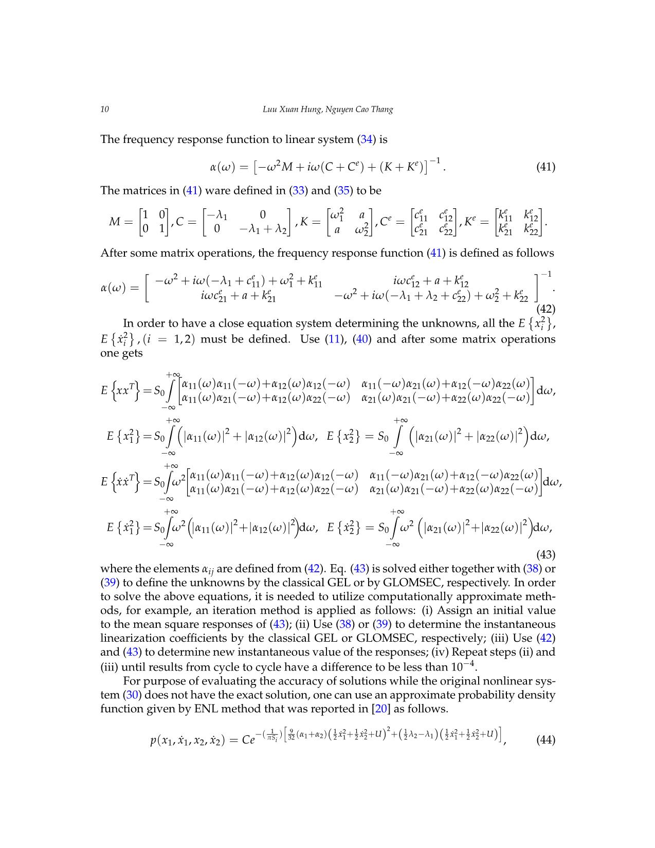
The frequency response function to linear system (34) is
−1
α(ω) = −ω2 M + iω(C + Ce) + (K + Ke) . (41)
The matrices in (41) ware defined in (33) and (35) to be
2 e e e e
1 0 −λ1 0 ω1 a e c11 c12 e k11 k12
M = , C = , K = 2 , C = e e , K = e e .
0 1 0 −λ1 + λ2 a ω2 c21 c22 k21 k22
After some matrix operations, the frequency response function (41) is defined as follows
2 e 2 e e e −1
−ω + iω(−λ1 + c11) + ω1 + k11 iωc12 + a + k12
α(ω) = e e 2 e 2 e .
iωc21 + a + k21 −ω + iω(−λ1 + λ2 + c22) + ω2 + k22
(42)
2
In order to have a close equation system determining the unknowns, all the E xi ,
2
E x˙i , (i = 1, 2) must be defined. Use (11), (40) and after some matrix operations
one gets
+
Z ∞
n To α11(ω)α11(−ω)+α12(ω)α12(−ω) α11(−ω)α21(ω)+α12(−ω)α22(ω)
E xx = S0 dω,
α11(ω)α21(−ω)+α12(ω)α22(−ω) α21(ω)α21(−ω)+α22(ω)α22(−ω)
−∞
+ +
Z ∞ Z ∞
2 2 2 2 2 2
E x1 = S0 |α11(ω)| + |α12(ω)| dω, E x2 = S0 |α21(ω)| + |α22(ω)| dω,
−∞ −∞
+
Z ∞
n To 2 α11(ω)α11(−ω)+α12(ω)α12(−ω) α11(−ω)α21(ω)+α12(−ω)α22(ω)
E x˙x˙ = S0 ω dω,
α11(ω)α21(−ω)+α12(ω)α22(−ω) α21(ω)α21(−ω)+α22(ω)α22(−ω)
−∞
+ +
Z ∞ Z ∞
2 2 2 2 2 2 2 2
E x˙1 = S0 ω |α11(ω)| +|α12(ω)| dω, E x˙2 = S0 ω |α21(ω)| +|α22(ω)| dω,
−∞ −∞
(43)
where the elements αij are defined from (42). Eq. (43) is solved either together with (38) or
(39) to define the unknowns by the classical GEL or by GLOMSEC, respectively. In order
to solve the above equations, it is needed to utilize computationally approximate meth-
ods, for example, an iteration method is applied as follows: (i) Assign an initial value
to the mean square responses of (43); (ii) Use (38) or (39) to determine the instantaneous
linearization coefficients by the classical GEL or GLOMSEC, respectively; (iii) Use (42)
and (43) to determine new instantaneous value of the responses; (iv) Repeat steps (ii) and
(iii) until results from cycle to cycle have a difference to be less than 10−4.
For purpose of evaluating the accuracy of solutions while the original nonlinear sys-
tem (30) does not have the exact solution, one can use an approximate probability density
function given by ENL method that was reported in [20] as follows.
1 h 9 1 2 1 2 2 1 1 2 1 2 i
−( πS ) 32 (α1+α2)( 2 x˙1+ 2 x˙2+U) +( 2 λ2−λ1)( 2 x˙1+ 2 x˙2+U)
p(x1, x˙1, x2, x˙2) = Ce i , (44)
Performance analysis of global-local mean square error criterion of stochastic linearization for nonlinear oscillators 11
where U(x1, x2) is the potential energy of the system.
1 1 b
U(x , x ) = ω2x2 + ω2x2 + ax x + (x − x )4 , (45)
1 2 2 1 1 2 2 2 1 2 4 1 2
and C is the normalization constant defined by
" #−1
Z ∞ Z ∞ 1 h 9 1 2 1 2 2 1 1 2 1 2 i 2
−( πS ) 32 (α1+α2)( 2 x˙1+ 2 x˙2+U) +( 2 λ2−λ1)( 2 x˙1+ 2 x˙2+U)
C = ... e i ∏ dxidx˙i . (46)
−∞ −∞ i=1
2
The mean square responses E xi NL obtained by ENL are
Z ∞ Z ∞ 1 h 9 1 2 1 2 2 1 1 2 1 2 i 2
2 2 −( ) (α1+α2)( x˙ + x˙ +U) +( λ2−λ1)( x˙ + x˙ +U)
= πSi 32 2 1 2 2 2 2 1 2 2
E xi NL C ... xi e ∏ dxidx˙i.
−∞ −∞ i=1
(47)
Consider two cases of the given parameters. Tabs.1 and2 show the mean square
responses of x1, x2 as well as their relative errors to solutions by ENL method (see also
Figs.1 and2).
Table 1. The mean squares of x1, x2 versus α (α1 = α2 = α) while λ1 = λ2 =
ω1 = ω2 = a = b = S0 = 1
n 2o n 2o ErrC n 2o ErrGL n 2o n 2o ErrC n 2o ErrGL
α1, α2 E x1 E x1 E x1 E x2 E x2 E x2
NL C |%| GL |%| NL C |%| GL |%|
0.1 1.57273 1.21597 22.684 1.40692 10.543 1.57273 1.15079 26.829 1.32675 15.640
1 0.49622 0.42145 15.068 0.48835 1.586 0.49622 0.36966 25.505 0.41930 15.501
5 0.25327 0.21986 13.191 0.25395 0.268 0.25327 0.20466 19.193 0.23409 7.573
10 0.19437 0.17091 12.070 0.19735 1.533 0.19437 0.16233 16.484 0.18625 4.178
Table 2. The mean squares of x1, x2 versus b while λ1 = λ2 = ω1 = ω2 =
a = α1 = α2 = S0 = 1
n 2o n 2o ErrC n 2o ErrGL n 2o n 2o ErrC n 2o ErrGL
b E x1 E x1 E x1 E x2 E x2 E x2
NL C |%| GL |%| NL C |%| GL |%|
1 0.49622 0.42145 15.068 0.48835 1.586 0.49622 0.36966 25.505 0.41928 15.505
10 0.36492 0.29566 18.980 0.33460 8.309 0.36492 0.29040 20.421 0.32769 10.202
50 0.33076 0.28086 15.086 0.31644 4.329 0.33076 0.28048 15.201 0.31597 4.472
100 0.32340 0.27930 13.636 0.31453 2.743 0.32340 0.27920 13.667 0.31440 2.783
From the relative errors of the approximate solutions with respect to the ones by
ENL, it can be seen that GLOMSEC gives a significant improvement on accuracy of solu-
tion in comparison with the classical GEL, especially when the nonlinearity is strong.
PerformancePerformance analysis of Global--LocalLocal
MeanMean SquareSquare ErrorError CriterionCriterion of stochastic linearization forfor nonlinearnonlinear oscillatorsoscillators
Table 2. The mean squares of xx, versus b while 1 2 1 2 aS 1 2 0 1
Table 2. The mean squares of xx1212, versus b while 1 2 1 2 aS 1 2 0 1
2 2 Err 2 Err 2 2 Err 2 Err
Ex2 Ex2 ErrCC Ex2 ErrGL Ex2 Ex2 ErrCC Ex2 ErrGLGL
b Ex 11NL Ex 11C Ex 1 GL Ex 22NL Ex 22C Ex 22GL
b NL C % GL % NL C % GL %
% % % %
11 0.496220.49622 0.421450.42145 15.06815.068 0.488350.48835 1.586 0.49622 0.369660.36966 25.50525.505 0.419280.41928 15.50515.505
1010 0.364920.36492 0.295660.29566 18.98018.980 0.334600.33460 8.309 0.36492 0.290400.29040 20.42120.421 0.0.3232769769 10.20210.202
5050 0.330760.33076 0.280860.28086 15.08615.086 0.316440.31644 4.329 0.33076 0.280480.28048 15.20115.201 0.315970.31597 4.4724.472
100100 0.323400.32340 0.279300.27930 13.63613.636 0.314530.31453 2.743 0.32340 0.279200.27920 13.66713.667 0.314400.31440 2.7832.783
12 Luu Xuan Hung, Nguyen Cao Thang
Figure 1. The mean square of x versus
FigureFig. 11.. TheThe mean mean square square of xof1 versusx11 versusα
FigureFig. 22.. TheThe mean mean square square of ofx2 versusx2 versusα
Figure 2. The mean square of x2 versus
4. CONCLUSION
This paper presents the proposed criterion with its algorithm built to MDOF nonlin-
ear oscillators under Gaussian white noise excitation. The mode of formulating algorithm
is also mainly based on the classical GEL. However, a key problem is to determine the
Performance analysis of global-local mean square error criterion of stochastic linearization for nonlinear oscillators 13
matrix of equivalent linearization coefficients in which the constant linearization coeffi-
cients are defined as global mean values of all local linearization coefficients. The paper
is an additional research to our previous ones [14, 15] to aim at evaluating the improved
performance of the proposed criterion; herein we analyse two applications, which are a
rolling ship oscillation and two-degree-of-freedom one. The results show a significant
improvement on accuracy of solutions by GLOMSEC in comparison with the ones by the
classical GEL.
ACKNOWLEDGMENTS
The paper is supported by Vietnam National Foundation for Science and Technology
Development (NAFOSTED) under grant number 107.04-2018.12.
REFERENCES
[1] T. K. Caughey. Equivalent linearization techniques. The Journal of the Acoustical Society of
America, 35, (11), (1963), pp. 1706–1711. https://doi.org/10.1121/1.1918794.
[2] T. K. Caughey. Response of a nonlinear string to random loading. Journal of Applied Mechanics,
26, (3), (1959), pp. 341–344.
[3] L. Socha. Linearization methods for stochastic dynamic systems. Lecture Notes in Physics,
Springer, Berlin, (2008).
[4] X. Zhang, I. Elishakoff, and R. Zhang. A stochastic linearization technique based on mini-
mum mean square deviation of potential energies. Stochastic Structural Dynamics, 1, (1991),
pp. 327–338. https://doi.org/10.1007/978-3-642-84531-4 17.
[5] F. Casciati, L. Faravelli, and A. M. Hasofer. A new philosophy for stochastic equiv-
alent linearization. Probabilistic Engineering Mechanics, 8, (3-4), (1993), pp. 179–185.
https://doi.org/10.1016/0266-8920(93)90013-l.
[6] N. D. Anh and W. Schiehlen. New criterion for Gaussian equivalent linearization. European
Journal of Mechanics - A/Solids, 16, (6), (1997), pp. 1025–1039.
[7] C. Proppe, H. J. Pradlwarter, and G. I. Schueller.¨ Equivalent linearization and Monte Carlo
simulation in stochastic dynamics. Probabilistic Engineering Mechanics, 18, (1), (2003), pp. 1–
15. https://doi.org/10.1016/s0266-8920(02)00037-1.
[8] I. Elishakoff, L. Andriamasy, and M. Dolley. Application and extension of the stochas-
tic linearization by Anh and Di Paola. Acta Mechanica, 204, (1-2), (2009), pp. 89–98.
https://doi.org/10.1007/s00707-008-0014-x.
[9] R. N. Iyengar. Higher order linearization in non-linear random vibration. International Jour-
nal of Non-Linear Mechanics, 23, (5-6), (1988), pp. 385–391. https://doi.org/10.1016/0020-
7462(88)90036-4.
[10] N. D. Anh and M. Di Paola. Some extensions of Gaussian equivalent linearization. In Pro-
ceedings of International Conferenceon Nonlinear Stochastic Dynamics, Hanoi, Vietnam, (1995).
pp. 5–16.
[11] N. D. Anh and L. X. Hung. An improved criterion of Gaussian equivalent linearization
for analysis of non-linear stochastic systems. Journal of Sound and Vibration, 268, (1), (2003),
pp. 177–200. https://doi.org/10.1016/s0022-460x(03)00246-3.
[12] N. D. Anh. Duality in the analysis of responses to nonlinear systems. Vietnam Journal of Me-
chanics, 32, (4), (2010), pp. 263–266. https://doi.org/10.15625/0866-7136/32/4/294.
[13] N. D. Anh. Dual approach to averaged values of functions. Vietnam Journal of Mechanics, 34,
(3), (2012), pp. 211–214. https://doi.org/10.15625/0866-7136/34/3/2361.
14 Luu Xuan Hung, Nguyen Cao Thang
[14] N. D. Anh, L. X. Hung, and L. D. Viet. Dual approach to local mean square error crite-
rion for stochastic equivalent linearization. Acta Mechanica, 224, (2), (2013), pp. 241–253.
https://doi.org/10.1007/s00707-012-0751-8.
[15] N. D. Anh, L. X. Hung, L. D. Viet, and N. C. Thang. Global–local mean square error criterion
for equivalent linearization of nonlinear systems under random excitation. Acta Mechanica,
226, (9), (2015), pp. 3011–3029. https://doi.org/10.1007/s00707-015-1332-4.
[16] J. B. Roberts and P. D. Spanos. Random vibration and statistical linearization. Wiley, New York,
(1990).
[17] J. B. Roberts. A stochastic-theory for non-linear ship rolling in irregular seas. Journal of Ship
Research, 26, (4), (1982), pp. 229–245.
[18] J. B. Roberts and N. M. C. Dacunha. Roll motion of a ship in random beam waves: Compari-
son between theory and experiment. Journal of Ship Research, 29, (1985), pp. 112–126.
[19] D. C. Polidori, J. L. Beck, and C. Papadimitriou. A new stationary PDF approximation for
non-linear oscillators. International Journal of Non-Linear Mechanics, 35, (4), (2000), pp. 657–
673. https://doi.org/10.1016/s0020-7462(99)00048-7.
[20] C. W. S. To. Nonlinear random vibration: Analytical techniques and applications. CRC Press,
(2011).
APPENDIX
T
Suppose that the components of the vector x = (x1, x2,..., xn) are zero-mean sta-
tionary Gaussian random variables. Denote E{.} global mean values of random variables
taken as follows
+ +
Z ∞ Z ∞
E {.} = ... (.) p (x)dx1dx2 . . . dxn, (A.1)
−∞ −∞
where p(x) is the stationary joint probability density function. For the Gaussian random
processes with zero mean, one has the following general expressions for expectations [2]
!
E {x1x2 ... x2n+1} = 0, E {x1x2 ... x2n} = ∑ ∏ E xixj , (A.2)
all dependent pairs i6=j
where the number of independent pair is equal to (2n)!/(2nn!) For example,
E {x1x2x3} = 0,
E {x1x2x3x4} = E {x1x2} E {x3x4} + E {x2x3} E {x1x4} + E {x1x3} E {x2x4} , (A.3)
E {x1x2x3x4x5} = 0.
If xi and xj (i 6= j) are uncorrelated, i.e. independent, then E{xixj} = 0, and
2n+1 2m+1
E{xi xj } = 0. Besides, formula (A.2) results in the following consequences
m
n 2n 2mo 2n n 2mo � 2 n n 2o
E xi xj = E xi E xj = (2n − 1)!! E xi (2m − 1)!! E xj , (A.4)
where n and m are natural numbers. Denote [.] the local mean values of random variables
taken as follows.
+rσ +rσ
Z x1 Z xn
E [.] = ... (.)p(x)dx1dx2 . . . dxn, (A.5)
−rσx1 −rσxn
Performance analysis of global-local mean square error criterion of stochastic linearization for nonlinear oscillators 15
where σx1, σx2 ..., σxn are the normal deviations of random variables, respectively, and
r is a given positive value. Due to the symmetry of the expected integrations in (A.5),
hereby (A.2) are also applied to the local mean values. If xi and xj (i 6= j) are uncorrelated,
h 2n+1 2m+1i
i.e. independent, then E xixj = 0, and E xi xj = 0. All higher even-order local
h 2n 2mi 2
means E xi xj can be expressed in terms of second order global means E xi and
n 2o
E xj as follows [16].
m
h 2n 2mi 2n h 2mi � 2 n n 2o
E xi xj = E xi E xj = 2Tn,r E xi 2Tm,r E xj , (A.6)
where
r r
Z Z
2n 2m 1 −t2 2
Tn,r = t η(t)dt, Tm,r = t η(t)dt, η(t) = √ e / . (A.7)
2π
0 0
If n = 0, m 6= 0 or n 6= 0, m = 0, then (A.6) leads to the following results, respectively
r
m Z
h 0 2mi n 2o h 2n 0i � 2 n
E xi xj = 2T0,r2Tm,r E xj , E xi xj = 2Tn,r E xi 2T0,r with T0,r = η(t)dt.
0
(A.8)
If r → ∞,(A.5) and (A.7) will give the same result as (A.4) of the classical case.
2
A local mean of xi |xi| that arises in an application of the paper was presented in [15],
the obtained result as follows
+rσ +rσ
Z xi Z xi
2 2 3
E xi |xi| = xi |xi| p(xi)dxi = 2 xi p(xi)dxi
−rσxi 0
r r
Z 1 2 2 2 Z
3 3 −t σxi/2σxi 3 3
= 2 t σxi √ e σxidt =2σxi t η(t)dt, (A.9)
2πσxi
0 0
r
Z
2 � 2 3/2 3
E xi |xi| = 2Tt3,r E xi , Tt3,r = t η(t)dt.
0
T T
If x = (x1, x2,..., xn) is the displacement vector, then x˙ = (x˙1, x˙2,..., x˙n) is the ve-
locity vector and we also obtain the same formulas, respectively, for the random variables
of velocity.File đính kèm:
 performance_analysis_of_global_local_mean_square_error_crite.pdf

